Python Data Analysis Library
In a previous session we explored NumPy in detail, learning about array structures and vectorisation. While NumPy is extremely powerful, it has some limitations. For example, data is organised into rows and columns (often in more than 2 dimensions) without labels other than indices. It is really hard to keep track of complex datasets by indexing and slicing alone – we need human-readable labels to make advanced queries and interpret complex results. This is where Pandas comes in – it is an invaluable tool for analysing labelled data. It takes data from csv, tsv, SQL or numerous other sources and converts it into a Python object ordered in rows and columns and persists the row and column labels, which can then be used to query the dataset.
Pandas should already be installed in your conda environment, so we can simply import using the convention:
import pandas as pd
1 DataFrames
1.1 DataFrame structure
The Pandas dataframe is a structure for storing data in 2D rectangular grids in which each column is a vector containing values for a particular variable. Within a row, there can be different types of data because the dtype is set column-wise and each column is a separate vector. A basic definition of a Pandas dataframe could be:
A labelled 2D data structure where each column, but not necessarily each row, contains a single dtype
Each value has an index, similarly to a NumPy array, but the Pandas dataframe also has named fields, meaning the data can be queried using names assigned by the user instead of keeping track of indices.
For example, let’s instantiate a dataframe named DF with columns named A, B and C, and add some data.
import numpy as np

DF = pd.DataFrame(columns=['A','B','C'])

array1 = np.random.randint(100,size=100)
array2 = np.random.randint(100,size=100)
array3 = np.random.randint(100,size=100)

DF['A'] = array1
DF['B'] = array2
DF['C'] = array3
One important point that you may already have noticed is that the dataframe can accept NumPy arrays. In this case we have provided three 1D NumPy arrays, effectively providing three vectors to become three columns in the dataframe, but we could also have provided a single 2D array:
import numpy as np

array1 = np.random.randint(30,size=(10,3))

DF = pd.DataFrame(array1,columns=['A','B','C'])
Just like with NumPy arrays, we can query the shape and size of the dataframe to understand the data dimensionality…
print("DF shape = ", DF.shape)
print("DF size = ", DF.size)
DF shape =  (10, 3)
DF size =  30
We can peek at the structure of this dataframe using the head() function which reports the top 5 rows of the dataframe to the console. This is really useful for checking quickly, by eye, that the column order, column labels, and dataframe orientation are correct, and that the values are consistent, correctly positioned and within an expected range.
DF.head()
We can also do the same for the final 5 rows in the dataframe using df.tail()
DF.tail()
We can also quickly access summary info about the dataframe structure using the df.info() function.
DF.info()
We can access columns using square brackets, similarly to indexing into NumPy arrays, but parsing the column name instead of its position in the matrix. For example, lets extract column A to a new variable. We expect that this will provide us with a vector of integers with a length of 10:
A = DF['A']
print("Shape of A = ",A.shape)
print("dtype = ", A.dtype)
print()
A.head()
Shape of A =  (10,)
dtype =  int64
1.2 DataFrames from files
In the example above we provided a NumPy array as input to the Pandas dataframe. As a data scientist you will likely need to use data stored externally in files such as .csv or .tsv (comma separated or tab separated values) or perhaps files from Excel or an SQL, NoSQL or MongoDB database, or some other file type. To begin with we will look at csv files. I have downloaded a csv file from Kaggle for this exercise and made it available in the notebook working directory. (https://www.kaggle.com/carlolepelaars/toy-dataset/). The dataset has 6 columns showing population data for 150,000 residents of Dallas, USA. Since it is a dataframe of population data, we’ll name it popDF.
popDF = pd.read_csv('./toy_dataset.csv')
print("Population dataframe has {} columns and {} rows ".\
format(popDF.shape[1],popDF.shape[0]))

popDF.head()
Rows and columns in Pandas datasets are often referred to differently, especially in the context of machine learning and data modelling. Columns are data “features” while the rows are “instances” of the features.
2 Exploratory Data Analysis
Pandas is an excellent tool for exploring a dataset because the dataframe structure promotes complex querying and there are many built in functions for exploration and visualization.
2.1 df.describe()
The data contained within the dataframe can be summarised using the pandas function describe(). This provides summary statistics for each column, including the number of rows (count), the mean, standard deviation, min and interquartile range of the values in that column. Notice that only the columns containing numeric data are included.
popDF.describe()
Notice that popDF.describe() only returned a summary of those columns containing numeric data. We can force the method to summarise other data types using the “include” keyword argument. In this case, where the operations are only achievable for numeric data types, a NaN is returned. Similarly, some new rows are added that provide summary values for non-numeric data and columns containing numeric dtypes simply return NaNs. These new columns show the number of unique entries in the column (“unique”), the most commonly occurring value (“top”) and that top value’s frequency of occurrence (“freq”).
popDF.describe(include=['object', 'float', 'int'])
We can also constrain the describe() method to a single column or a set of columns
popDF['Age'].describe() #describe only the Age column
popDF[['Age','Income']].describe()
2.2 More info
The structural information about the dataframe is accessible using df.info()
popDF.info()
For the non numeric dtypes, we can query the frequency of each unique value in the dataframe using value_counts(), for example, how many instances are there for each city?
popDF['City'].value_counts()
We can also report these data as proportions of the total rather than absolute count values…
popDF['City'].value_counts(normalize=True)
2.3 Sorting and reformatting
We can sort the data using the built-in sort function. By default the data is sorted into ascending order (smallest first), to sort into descending order (largest first) we can set the argument ascending = True.
# sort values by income, in descending order, and display the top 5 rows

popDF.sort_values(by='Income', ascending=False).head()
Sorting by multiple columns is also possible. For example, sorting by income (descending) and age (ascending) results in a dataset where the youngest, richest instance is at the top of the dataframe. The algorithm will osrt by income first, then sort rows with matching income by the age. Therefore, the result of sorting by both columns will be identical to sorting only by income unless there are rows with identical income values.
popDF.sort_values(by=['Income', 'Age'],ascending=[False, True]).head()
We can further demonstrate this by using a non-numeric dtype as one of the sort criteria. For example, if we sort by City first, then income, we will get a dataframe with the residents of each city (alphabetical order) ordered by their income.
popDF.sort_values(by=['City', 'Income'], ascending=[True, False]).head()
It can sometimes be useful to change the dtype of a particular column. We can do this using the built-in .astype() function.
popDF['Number'] = popDF['Number'].astype('float64')   # change Number column to float64

popDF['Number'].describe()  # check result
3 Indexing and Multi-indexing
3.1 Indexing
There are several options for indexing data in Pandas. While NumPy only allows numerical indexing using the column and row numbers, Pandas allows data to be selected using row and column labels. Label-based indexing of columns can be achieved simply by passing a column label in square brackets:
# This will grab the column "City" from popDF and assign it to the variable "CityColumn"

CityColumn = popDF['City']
CityColumn.head()
The syntax is the same for multiple columns:
# This will grab the "City" and "Gender" columns and assign them both to the variable "CityAndGenderColumns"

CityAndGenderColumns = popDF[['City','Gender']]

CityAndGenderColumns.head()
3.1.1 df.loc[ ]
The .loc[] function exists for extracting rows from a DataFrame using index labels. Our DataFrame currently has integer indexes (0,1,2,3) so here we can create a small example DataFrame using just the first five rows from popDF and replace the index labels with text labels.
# first grab the first 5 rows of popDF and assign the small DataFrame to variable "smallDF"

smallDF = popDF.head()

# replace the integer indexes in smallDF with text labels

smallDF.index=['one','two','three','four','five']
Now we have an example DataFrame with each row indexed with a text label. We can now demonstrate the .loc[] function for selecting data by text labels. We pass the row label to .loc[] and the result is the values of all columns in the DataFrame for the selected row:
# select row three

smallDF.loc['three']
This can also be applied to selecting multiple rows:
# select rows one and three

smallDF.loc[['one','three']]
or it can be applied to selecting ranges of rows. For example, let’s select all rows between two named rows.
# select roIndexingws between one and three

smallDF.loc['one':'three']
It is also valid to pass a condition that creates a Boolean array to .loc[]. For example, the statement popDF.loc[‘Gender’]==”Female’ returns a Boolean array where those rows where ‘Female’ exists in the ‘Gender’ column contain ‘True’ and the others contain ‘False’. The rows containing ‘True’ are selected.
# Select rows where Age is equal to 41

smallDF.loc[smallDF['Age']==41]
Specific row values in certain columns can be selected by adding arguments to .loc[]. In the example below we extract the City and Gender values ony for rows where the Age is equal to 41.
smallDF.loc[smallDF['Age']==41,['City','Gender']]
3.1.2 df.iloc[ ]
An alternative to .loc[] is .iloc[]. This is used for indexing by integer values instead of text labels, replicating the numerical indexing syntax from NumPy. To demonstrate we can switch back to using popDF.
# select first row from dataframe

popDF.iloc[0]
# select rows 10 to 15 from dataframe

popDF[10:15]
# select fifth to tenth rows from Age column (4th column)

popDF.iloc[5:11,3]
# select fifth to tenth rows from Gender, Age and Income columns

popDF.iloc[5:11,[2,3,4]]
There are some interesting potential gotchas to consider with .loc[]. You may have noticed in the previous cells that when a single row is selected it is displayed differently (a vertical arrangement of plain text) compared to multiple rows (a neatly presented and formatted as a table). This is because when only one row is selected .iloc[] returns a Pandas Series object. To maintain the DataFrame type, .iloc[] requires a single valued list to be passed.
#print the type of the object returned by .iloc[] when a row value is passed

print(type(popDF.iloc[500]))

popDF.iloc[500]
<class 'pandas.core.series.Series'>
# print the type of the object returned by .iloc[] when a single-valued list is passed

print(type(popDF.iloc[[500]]))

popDF.iloc[[500]]
<class 'pandas.core.frame.DataFrame'>
3.2 Heirarchical indexing/ Multi-indexing
Heirarchical indexing is the method used by Pandas to represent multidimensional data. Note that for most purposes, data with >2 dimensions is better analysed using the Python package “xarray”. However, multi-indexing enables Pandas to force multidimensional data into a two-dimensional structure. This allows that data to be analysed in Pandas. The concept underpinning multi-indexing is the ability to represent n-dimensional data in lower dimensional Series and DataFrame structures.
Our population dataset fits nicely into a two dimensional structure with rows and columns, but what about if we wanted to capture changes in the same variables over time? In this case, we need to label each element with a date as well as a row and column index. Each element therefore has a position in three dimensions – row, column and a third ‘time’ dimension. Multi-indexing allows this to be captured without breaking the two-dimensionality of the Pandas DataFrame.
In the following example, we consider the populations of the cities included in our popDF DataFrame in two succesive years – 2019 and 2020. To achieve this, we first define an index. We want to be able to index the data by both the city name and the year, so that we can extract Los Angeles in 2019, for example.
I have made up the population values below. They are assembled into a Pandas DataFrame and the index is a list of tuples detailing the city name and year.
# Define the values to be used as indexes - this should be a list of tuples where each tuple contains the
# city name and year

index = [('Dallas', 2019), ('Dallas', 2020), ('New York City', 2019), ('New York City',2020),
         ('Los Angeles', 2019),('Los Angeles', 2020), ('Mountain View', 2019),('Mountain View', 2020),
         ('Boston', 2019), ('Boston', 2020), ('Washington D.C.', 2019), ('Washington D.C.', 2020),
         ('San Diego',2019), ('San Diego', 2020), ('Austin',2019), ('Austin', 2020)]

## define the populations of each city in each year (the order must be consistent with the tuples in index)

population = [32423452, 35554326, 45456751, 44123454, 55090987,56789033, 18976457, 19378102, 20851820,
              25145561, 65453674, 65380987, 34545643, 34876758, 4563355, 47649094]

# create a Pandas MultiIndex object from the list of tuples

index = pd.MultiIndex.from_tuples(index)

# create a DataFrame with the populations as the data and the MultiIndex object 'index' as the index

multiDF = pd.DataFrame(population,index=index)

# rename the column

multiDF.columns=['population']
If we display the content of the new multi-indexed dataframe we can see that each “city” index label has associated with it two “year” indexes.
# display the contents of the multi-indexed dataframe

multiDF
| population | ||
|---|---|---|
| Dallas | 2019 | 32423452 |
| 2020 | 35554326 | |
| New York City | 2019 | 45456751 |
| 2020 | 44123454 | |
| Los Angeles | 2019 | 55090987 |
| 2020 | 56789033 | |
| Mountain View | 2019 | 18976457 |
| 2020 | 19378102 | |
| Boston | 2019 | 20851820 |
| 2020 | 25145561 | |
| Washington D.C. | 2019 | 65453674 |
| 2020 | 65380987 | |
| San Diego | 2019 | 34545643 |
| 2020 | 34876758 | |
| Austin | 2019 | 4563355 |
| 2020 | 47649094 |
With this structure we can simply index into the multi-indexed DataFrame using the normal .loc syntax, for example let’s extract the population for Dallas in 2019…
With this structure we can simply index into the multi-indexed DataFrame using the normal .loc syntax, for example let’s extract the population for Dallas in 2019…
multiDF.loc['Dallas',2019]

population    32423452
Name: (Dallas, 2019), dtype: int64
or all of the population data for Dallas:
multiDF.loc['Dallas',:]
or the population data for all cities in 2020…
multiDF['population'].loc[:,2020]
We can also reformat this into a more intuitive two dimensional representation with two sub-columns beneath population, one for each year. This is achieved by ‘unstacking’ the dataframe using df.unstack()…
multiDF.unstack()
It is also possible to specify which level to unstack, for example, unstacking the first index (City) creates a two dimensional structure with separate columns for each city, with the years remaining as row indexes:
multiDF.unstack(level=0)
Alternatively, we could unstack the second index, giving columns for years. This is what occurred by default when we did not specify a level to unstack.
multiDF.unstack(level=[1])
We can also completely unstack the dataframe by specifying both levels. In this case, the structure returned is a Pandas Series object. This makes sense because each unstack effectively removes a dimension from the structure – a multi-indexed dataframe with two indexes (which can be conceptualized as a three dimensional structure) is reduced to a flat two-dimensional dataframe when it is unstacked on one level. Unstacking another dimension effectively removes the indexes, reorganising the data into one dimensional lists.
multiDF.unstack(level=[0,1])
It is important to note that some multi-indexing slicing methods will fail if the indexes are not sorted, so the pd.sort_index() function cna be used to ensure the indexes are sorted into numerical or alphabetical order:
multiDF = multiDF.sort_index()

multiDF
We can also apply operations over specific levels in a multi-indexed DataFrame. For example, perhaps we want to know the mean population in each city over all available years. In this case, we specify that the df.mean() function should operate over the first level.
multiDF.mean(level=0)
Alternatively, we might wish to see the mean across all cities for each year, in which case we specify the second level:

multiDF.mean(level=1)
4 Visualising Data
There are many ways to visualise data from Pandas using external plotting libraries such as matplotlib and seaborn, but there are also powerful visualisation functions built-in to Pandas. These are built on top of Matplotlib but are accessible via the Pandas API.
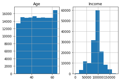
There are many plot types available in Pandas that are all accessed using very similar syntax. For example, there is a very useful built-in method for plotting histograms of data elements, using df.hist(). In the example below we plot histograms for Age and Income from the popDF DataFrame. Automatically, only those columns that have numeric data types are included, but in the example below I limit it to Age and Income.
# plot histogram using df.hist()

histogram = popDF[['Age','Income']].hist()
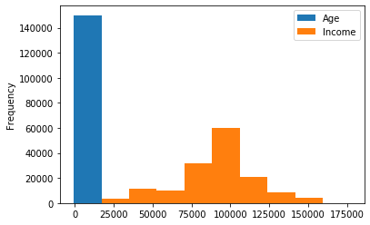
The histogram above was created using the .hist() function, but there is another more general route to achieving the same plot. This is to use the df.plot() function and pass kind = ‘hist’ as a keyword argument. The major difference between these two options is that the former allows the user to call .hist() once with multiple data elements and Pandas automatically produces a multi-panel plot with separate axes for each histogram. Using df.plot() returns a single axes object, so either multiple elements are plotted on the same axes or they are plotted separately, either by producing multiple figures or by manually constructing a multi-panel figure and individually assigning elements to specific panels.
# calling .plot(kind='hist') on multiple elements - all histograms share axes

popDF[['Age','Income']].plot(kind='hist')
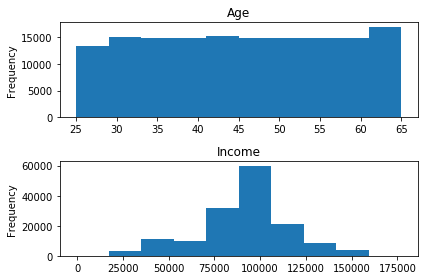
# manually constructing subplots with Matplotlib and assigning Pandas .plot objects to specific axes

import matplotlib.pyplot as plt

fig, axes = plt.subplots(nrows=2, ncols=1)

popDF['Age'].plot(kind='hist', ax=axes[0])
popDF['Income'].plot(kind='hist',ax=axes[1])
axes[0].set_title('Age')
axes[1].set_title('Income')
plt.tight_layout()
With either method, there are also many options for configuring the histogram, such as defining the number of bins…
histogram = popDF[['Age','Income']].hist(bins=80)

There are also many other types of data visualisation that can be achieved using the same basic syntax. The ‘kind’ kwarg is used to instruct Pandas to create a certain type of pot from a long list of options including line, bar, box, density, area, pie, scatter and more. If ‘kind’ is not defined in the call to df.plot(), Pandas defaults to a line plot.
# plot popDF['Age'] as a box plot

boxplot = popDF['Age'].plot(kind='box')

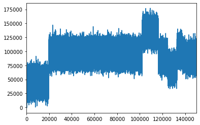
# plot popDF['Income'] as a line plot

lineplot = popDF['Income'].plot()

# this is equivalent to:

# lineplot = popDF['Income'].plot(kind='line')
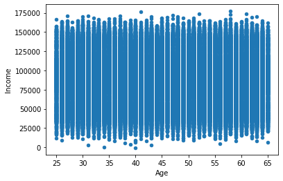
# scatter plot showing Age against Income

popDF.plot(kind='scatter',x='Age',y='Income')
We can also always combine plot types into a matplotlib subplots object…
# add a box plot, line plot, scatter plot and histogram to a multipanel figure

fig, axes = plt.subplots(figsize=(12,10),nrows=2, ncols=2)

popDF['Age'].plot(kind='hist', ax=axes[0,0])
popDF['Income'].plot(kind='box',ax=axes[0,1])
popDF['Age'].plot(kind='line',ax=axes[1,0])
popDF.plot(kind='scatter',x='Age',y='Income',ax=axes[1,1])

axes[0,0].set_title('Histogram of Age')
axes[0,1].set_title('Box plot of Income')
axes[1,0].set_title('Line plot of Age')
axes[1,1].set_title('Scatter plot of Age and Income')

plt.tight_layout()

5 Further Reading
This just scratched the surface of data analysis with pandas, there is lots more information out there that can take you much deeper into the Pandas package. I have not covered groupby functions, data transformations, sorting or filtering, and have only lightly touched on data i/o. I may well do some more notebooks covering those topics and others later, but for now here are some suggestions for further reading:
https://pandas.pydata.org/docs/index.html https://towardsdatascience.com/a-quick-introduction-to-the-pandas-python-library-f1b678f34673 https://jakevdp.github.io/PythonDataScienceHandbook/03.00-introduction-to-pandas.html https://towardsdatascience.com/learn-advanced-features-for-pythons-main-data-analysis-library-in-20-minutes-d0eedd90d086
